Weather Research and Forecasting (WRF) model/UNU 2010 Training
Important notes
- WRF system uses Universal Time for all its calculations.
Reading Material
- WRF Users site [1] has a number of publications that gives details of the theory, working and applications of the model. Particularly:
How your system runs
- WRF model does not run on windows operating system, it needs many advanced services provided by UNIX-like operating systems. We use Linux to run the modeling system.
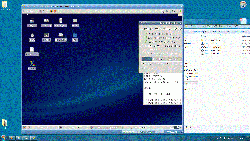
- It is possible to install Linux side-by-side with Windows on a PC. However, for this tutorial we take an alternative approach: We run Linux inside Windows! This is called Virtualization. We use the excellent virtualization software known as VMWare. VMWare is a free software (but not fully open source!) and shows excellent performance in running Linux within Windows Operating System. This is a technology that has been there for a number of years and a one that has matured to be quite usable in practice. In fact, many companies today, routinely use VMWare to run multiple operating systems in one physical computer.
Installation made easy
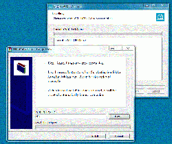
- I have provided a DVD-ROM Disk packed with all the tools that are necessary to run Linux on VMWare. Just push in the DVD to your computer and click on setup.exe.
- First select the option to install VMWare player.
- The installation program first installs VMWare Player on your hard disk (first phase).
- Usually the installer asks to reboot, please do so. This happens during VMWare Player software installation (first step of the DVD) After rebooting first let any automatically starting setup processes to continue.
- After successfully installing VMWare player, choose to install Java and WRF Domain Wizard. This installation is also easy like the above and takes only a few minutes.
- The final phase of the installation is installing the WRF_Linux system. It can take a long time. Your DVD drive needs to copy more than 4.5GB of data and your hard disk needs about 8GB data. So, be patient, please! It is normal to take much more than an hour for this in a slow computer.
- Please note that the WRF_LINUX system takes up a lot of space. You need at least 10GB of free disk space. If you have such space on a drive that is different from standard C: (say D:) then direct the installation program to that disk when prompted to install WRF LINUX.
How to use your system
As was mentioned before, WRF model is meant to be operated within a UNIX/Linux operating system. However, we'll attempt to run most of the pre-processing tasks from Windows (accessing your VMWare system remotely) and will venture into Linux (VMWare system) to do the actual model running and post-processing only. Make sure your share directory works properly. If not re-enable sharing and specify a share directory from Virtual Machine->Virtual Machine Settings-> Options->Shared Folders menu on top of you WMWare window. Shared folder is needed to exchange data between windows (host) and Linux (VMWare guest)
Running WRF
First login to the Linux system and check its IP address.
There is an icon on your desktop that will find this for you. Or you can use the command <tt>ifconfig</tt>.
(Note the IP address down. Also remember that this IP address can change each time
If you cannot connect to Linux from Domain Wizard, recheck the IP address.)

At this stage, you can minimize (do not close!!) VMWare window and return to windows system. Do the following on windows.


1. Run Domain Wizard (There is a shortcut in the WRF_LINUX start menu/Desktop entry).
2. Set up the connection as follows:
(First time you have to click on WPS program to initiate entering the following data)
      Computer: The IP address you noted down
      WPS Programs: /opt/wrf.run/WPS
      Geography: /home/wrf/geog
      Domains: /home/wrf/work
3. Read the section "idiosyncrasies of Domain Wizard". Then do the pre-processing (geogrid, ungrib,
metgrid) from within domain wizard.
4. Now go to the linux machine.

5. run mywrf_modelcopy.bash <domainname> from the directory of your domain (~/work/<yourdomainname>).
This will create a directory WRFV3 under it. Change directory to ./WRFV3/test/em_real
6. In the namelist.input make sure that if there is a entry dyn_opt under &dynamics the entry is
commented (!). This may be a bug in the system!
7. run ./real.exe, then check if the run is successfull (check the rsl* files)
8. If that is successful, then run WRF model by ./wrf.run.bash
9. Run mywrf_postplot.bash to check your output.
idiosyncrasies of Domain Wizard
when editing namelist.input in wrf domain wizard remember to change Run_Days, hours start end dates interval_seconds history_interval frames_per_outfile (large number) and REMEMBER to Save (Action -> Save)
In the Run Preprocessors page, link the grib files. REMEMBER to set the Grib start and end date/times according to namelist.input requirements. Then SAVE!!
If a domain is reopened using Domain Wizard. Never say yes to the question "Regenerate wrf.input" If you do, all your changes will be lost!!
Panoply
Currently panoply does not support dynamic zooming. Use the map tab of the created map to manually ajust scaling and centering. When good set it in Preferences. Panoply will use these settings in the future.
Notes: Remember the incompatibility of &dynamics section. However, the mywrf_modelcopy.bash takes care of this.
GRIB Files
Best place to put downloaded grib files is the share directory. Downloading can be done in windows. Just download the files and copy them to the share directory.
A good starting options for a WRF simulation
- Rainfall Microphysics (mp_physics) use Ferrier Scheme (option 5)
- Cumulus Parameterization (cu_physics) use Grell 3D (Option 5)
Flash Floods in Hannibal, Missouri -- Mark Twains Home Town
"The rain is famous for falling on the just and unjust alike, but if I had the management of such affairs I would rain softly and sweetly on the just, but if I caught a sample of the unjust out doors I would drown him" -- Mark Twain
- map [4]
- Vital data
- Date
- 20-Jul-2010
- Time of storm
- 0400 to 09:00 (Central Daylight Time). in Universal Time: 0900 to 1400 (UTC).
- Rainfall amounts
-
- Hannibal: 3.4 inches.
- Quincy: 2.1 inches.
- Palmyra: 2.8 inches.
- Monroe City: 5.5 inches.
- New London: 4. 4 inches
- Perry: 5. 3 inches.
- Saverton: 2.3 inches.
- Shelbyville: 8 inches.
- Bowling Green: 5.2 inches.
- Louisiana: 5 inches
Some good starting points -- NCAR's experience
(After NCAR, [5]) Examples of namelist for various applications A few physics options sets (plus model top and number of vertical levels) are provided here for reference. They may provide a good starting point for testing the model in your application. Also note that other factors will affect the outcome. For example, the domain setup, the distributions of vertical model levels, and input data. a. 1 – 4 km grid distances, convection-permitting runs for 1- 3 days run (as used for NCAR spring real-time convection forecast over US):
mp_physics                          = 8,
ra_lw_physics                       = 1,
ra_sw_physics                       = 2,
radt                                = 10,
sf_sfclay_physics                   = 2,
sf_surface_physics                  = 2,
bl_pbl_physics                      = 2,
bldt                                = 0,
cu_physics                          = 0,
ptop_requested                      = 5000,
e_vert                              = 35,
b. 20 – 30 km grid distances, 1- 3 day runs (e.g., NCAR daily real-time runs over US):
mp_physics                          = 4,
ra_lw_physics                       = 1,
ra_sw_physics                       = 2,
radt                                = 10,
sf_sfclay_physics                   = 2,
sf_surface_physics                  = 2,
bl_pbl_physics                      = 2,
bldt                                = 0,
cu_physics                          = 5,
cudt                                = 0,
ptop_requested                      = 5000,
e_vert                              = 30,
c. Cold region 15 – 45 km grid sizes (e.g. used in NCAR’s Antarctic Mesoscale Prediction System):
mp_physics                          = 4,
ra_lw_physics                       = 1,
ra_sw_physics                       = 2,
radt                                = 10,
sf_sfclay_physics                   = 2,
sf_surface_physics                  = 2,
bl_pbl_physics                      = 2,
bldt                                = 0,
cu_physics                          = 1,
cudt                                = 5,
fractional_seaice                   = 1,
seaice_threshold                    = 0.0,
ptop_requested                      = 1000,
e_vert                              = 44,
d. Hurricane applications (e.g. 12, 4 and 1.33 km nesting used by NCAR’s real-time hurricane runs):
mp_physics                          = 8,
ra_lw_physics                       = 1,
ra_sw_physics                       = 2,
radt                                = 10,
sf_sfclay_physics                   = 1,
sf_surface_physics                  = 1,
bl_pbl_physics                      = 1,
bldt                                = 0,
cu_physics                          = 1, (only on 12 km grid)
cudt                                = 5,
isftcflx                            = 2,
ptop_requested                      = 2000,
e_vert                              = 36,
e. Regional climate case at 10 – 30 km grid sizes (e.g. used in NCAR’s regional climate runs):
mp_physics                          = 6,
ra_lw_physics                       = 3,
ra_sw_physics                       = 3,
radt                                = 30,
sf_sfclay_physics                   = 1,
sf_surface_physics                  = 2,
bl_pbl_physics                      = 1,
bldt                                = 0,
cu_physics                          = 1,
cudt                                = 5,
sst_update                          = 1,
tmn_update                          = 1,
sst_skin                            = 1,
bucket_mm                           = 100.0,
bucket_J                            = 1.e9,
ptop_requested                      = 1000,
e_vert                              = 51,
spec_bdy_width                      = 10,
spec_zone                           = 1,
relax_zone                          = 9,
spec_exp                            = 0.33,

